In this post, I will show some simple experiments I ran to adjust the built in FET component of ngspice to model a particular FET. This follows up on this previous post where I showed how to install ngspice and run some preliminary experiments to model a zener diode’s behavior in a circuit.
The FET I chose is a standard one that seems used quite often It is the International Rectifier IRFP150N. Here is the datasheet.
Here is a simple netlist for a FET test. Put the following in a file called test_irfp150n.cir:
MOS OUTPUT CHARACTERISTICS
.OPTIONS NODE NOPAGE
VDS 3 0 50v
VGS 2 0 5v
M1 1 2 0 0 MOD1
* VIDS MEASURES ID, WE COULD HAVE USED VDS, BUT ID WOULD BE NEGATIVE
VIDS 3 1 0V
.model MOD1 NMOS ()
.DC VGS 4 10 1
.END
The interesting part of this file is that it is not a dynamic time-variant simulation. Instead, it is testing the circuit at various DC voltages for VGS. The line “.DC VGS 4 10 1” says “try this circuit out with varying values of VGS voltage from 4 to 10 stepping one volt at a time”.
So go ahead and run the file with:
ngspice test_irfp150n.cir
Now you can plot the current passing through the FET with the following commands:
run; plot i(vids)
You should see something like the following:

Notice that at 10V for VGS, we are seeing only 1mA of current passing through the FET. To be honest, I am really wondering why the defaults for FETs in ngspice are so strange. If you have any ideas, please let me know.
Now compare the VGS vs IDS current in the IRFP150N datasheet on page 3 (Fig 3). You can see that at 10V, we should be seeing about 100A. Going back to the MOSFET section of the ngspice User Manual we can look at the various parameters of the FET model that can be tweaked to get the behavior we want. In particular, KP (transconductance) is in units of A/V^2. By tweaking the KP, I found that a value of 2 gives a result of 100A at 10V for VGS. (Why is the default 2e-5?)
To try this out, simply change the “.model MOD1 NMOS ()” line (3rd line from the bottom) to read “.model MOD1 NMOS (KP=2)“. Then run:
source test_irfp150n.cir ; run; plot i(vids)

Now you can see that at VGS=10V, the current is 100A which is close to the datasheet. But at 4V, the current is about 17A vs the datasheet value of about 4A (simulation defaults to 27 degrees). To effect this change, we will play with the VTO parameter (Zero-bias threshold voltage).
Through trial and error, I was able to get the following parameters to have a IDS=4A at VGS=4V and IDS=100A at VGS=10V:
.model MOD1 NMOS (VTO=2.52 KP=3.65 )
giving us a current plot that looks like:
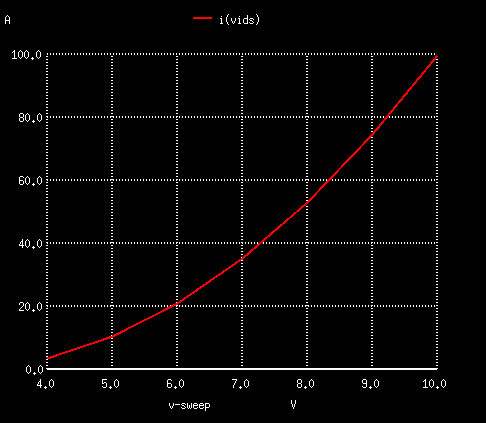
Now if you are wondering why it doesn’t look exactly like the current graph in the datasheet, that is because they graph it on a log scale. You can get that by running “plot log(i(vids))“:
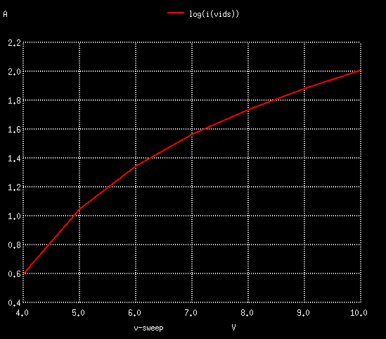
Since log10(4)=0.6 and log10(100)=2, this shows that we have reasonable end values at the 4V and 10V VGS. But now if we look at VGS=6, we see about 20A of current where the data sheet shows closer to 40A.
I’ll leave tuning that for a later date. Still a work in progress.